

California Zit-Pics
Spring: when posts showing cross-sections through massive California pimples bloom across LinkedIn

Following on from my California Battery Reality post I’ve applied my approach using CAISO data for four recent days highlighted in Prof. Mark Z Jacobson’s LinkedIn pustule-posts. For details of my methodology, see Appendix 1 below.
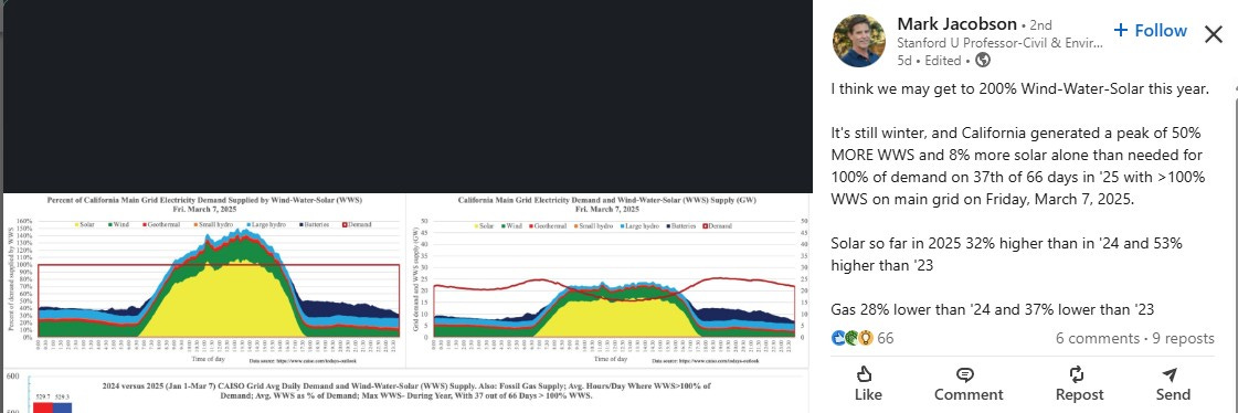
Figure 1: Jacobson Zit-Pics 6th March 2025:

Figures 1B: Thursday 6th March 2025 Energy Balances:


Definitely a decent Solar day: the average could be 5,745 MW every hour of the 24 (in the unlikely / very expensive future wherein sufficient immense BESS capacity is in place). However, on this day Natural Gas provided 114.5 thousand MWh (21%) of CA’s Demand while Solar provided 137.9 thousand MWh (25%) [not accounting for curtailment, if any]. Therefore, simply for Solar to displace gas requires Solar to be increased by a factor (137.9+114.5) / 137.9 = 1.83 = the ‘Solar increase required’.
My battery simulation shows the BESS requirement to smooth this day’s Solar power to 5,745 MW every hour is ~ 97,000 MWh ~ 33 times Moss Landing. Applying the ‘Solar increase required’ factor brings this up to
60 times Moss Landing
Actual CA batteries took 35.3 thousand MWh of electrical energy to charge, and discharged 27.2 thousand MWh back to the CAISO grid. In other words, just over
8 thousand MWh were lost due to cumulative battery system inefficiencies.
The implied round trip efficiency (RTE) is 77% on these recorded numbers.
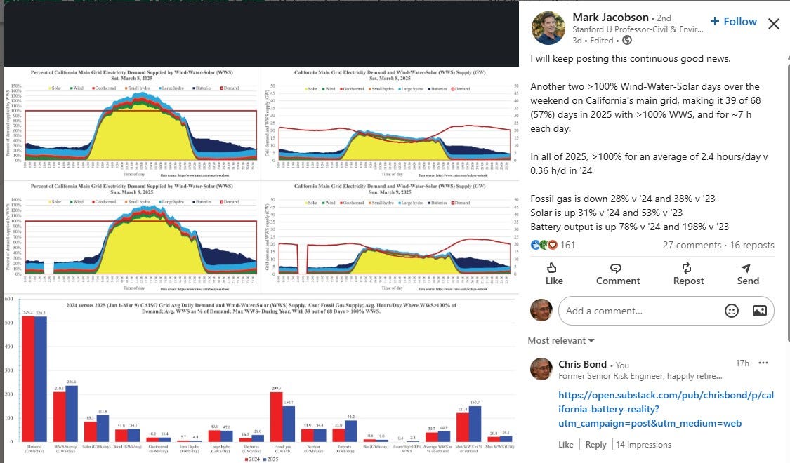
Figure 2: Jacobson Zit-Pics 7th March 2025:
Figures 2B: Friday 7th March 2025 Energy Balances:


An even better Solar day. The average could be 6,668 MW every hour of the 24 (… future wherein sufficient immense BESS capacity is in place). However, on this day Natural Gas provided 93.3 thousand MWh (18%) of CA’s Demand while Solar provided 160.0 thousand MWh (31%) [not accounting for curtailment, if any]. Therefore, simply for Solar to displace gas requires Solar to be increased by a factor (160.0+93.3) / 160.0 = 1.58 = the ‘Solar increase required’.
My battery simulation shows the BESS requirement to smooth this day’s Solar power to 6,668 MW every hour is ~ 114,000 MWh ~ 38 times Moss Landing. Applying the ‘Solar increase required’ factor again brings this up to
60 times Moss Landing
Actual CA batteries took 40.8 thousand MWh of electrical energy to charge, and discharged 36.1 thousand MWh back to the CAISO grid. In other words, nearly
5 thousand MWh were lost due to cumulative battery system inefficiencies.
The implied round trip efficiency (RTE) is 89% on these recorded numbers.
Figure 3: Jacobson Zit-Pics 8th-9th March 2025:
Figures 3B: Saturday 8th and Sunday 9th March 2025 Energy Balances:


Again, despite their good Solar showings, quite a lot of gas was burned on both days of that weekend despite lower Demands. This would require 1.61 and 1.53 factors more Solar respectively simply to displace that gas. The BESS capacity required to smooth the Solar across all 24 hours of each day to avoid massive extra curtailment is
57 to 60 times Moss Landing
Why is this energy storage capacity (of whatever technology) necessary? Because as California installs more Solar *capacity* it is forced to curtail ever more of the power that’s surplus to Demand simply to maintain grid stability.
Figures 4: CAISO Wind & Solar Curtailments, 2024:
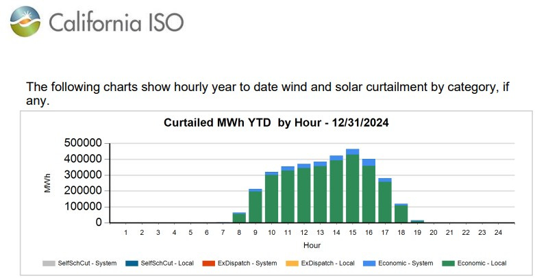
All that ‘free’ energy going to waste / not earning any return on all the capital expended on the Solar panels / inverters / cables / engineering / etc.
From the profiles of power Imports on each of these days, it doesn’t look to me like CA could export much more of its excess Solar power instead of curtailing it.
It could, instead of building enormous BESS capacity, build enormous additional Demand… providing that additional Demand is reliable / schedulable and flexible enough to be able to cope with the vagaries of weather-dependent generation.
Because the absolute electricity grid requirement, Supply = Demand, must be satisfied 60/24/365.
Otherwise California’s lights would go out.
Why I am ‘picking at Prof. Jacobson’s zits’
Because his propaganda posts don’t add anything to the debate around the difficult parts of ‘decarbonisation’. The phase where an x% increase in the *capacity* of ‘renewables’ leads to quite a lot less than x% increase in usable ‘renewable’ power because an increasing fraction of x% has to be curtailed.
That annoys me.
Appendix 1: Details of Methodology
I outline my methodology here for anyone interested.
1) CAISO Data Transposed into Columns:
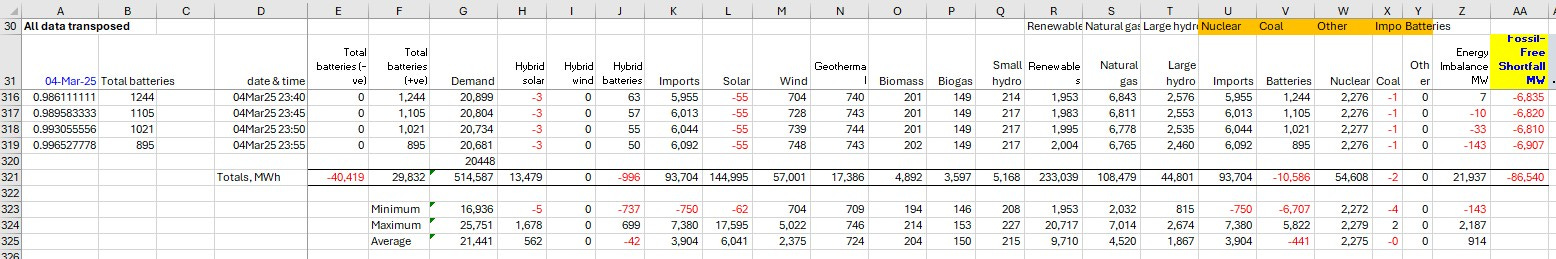
As I mentioned in my earlier post, six different downloads from CAISO (batteries; demand; hybrids; imports; renewables; supply) are required for each day. And all the CAISO comma-separated variable (.csv) files have the data arranged in rows not columns. That’s 288 columns across (5-minute data intervals) for each whole day.
I find it more clumsy to process the data when it is arranged in rows, so I used Excel’s Copy, then Paste Values Transpose to re-order the data into columns:
Column A is decimal time: added to the date and displayed Date & Time in Column D;
Column B is the “Total batteries” row of data CAISO transposed into column format;
Column C is left blank;
Column E is for all negative values of “Total batteries”, i.e. for battery charging;
Column F is for all positive values of “Total batteries”, i.e. for battery discharging to the CAISO grid;
Column G is the “Demand” row of CAISO data transposed into column format;
Columns H, I, J are the “Hybrid” rows of CAISO data transposed into column format;
Column K is the “Import” row of CAISO data transposed into column format;
Columns L thru Q are the “Renewables” rows of CAISO data transposed into column format;
and Columns R thru Y are the “Supply” rows of CAISO data transposed into column format… with the added twist that CAISO changed its data-file structure between my original post and now, swapping the Nuclear and Coal rows with the Other, Imports and Batteries rows. Hence I had to ensure I kept them in their correct columns for data processing and analysis. Which is why those column headings are highlighted in orange.
The “Totals” in row 321 are the arithmetic sum of all the MW values multiplied by 5/60 to get MWh for each column.
The “Minimum”, “Maximum” and “Average” values in rows 323, 324 and 325 are the Excel function =MIN(), =MAX() and =AVERAGE() results for each relevant column range e.g. =MIN(G32:G319) for minimum Demand.
2) Energy Imbalance (cross-check):
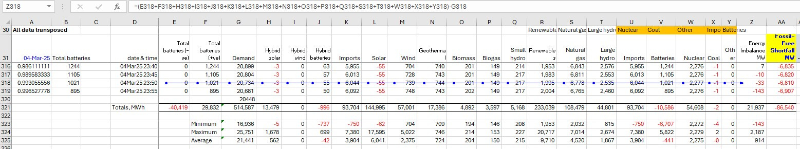
The “Energy Imbalance MW” in Column Z is the arithmetic sum of all the power supply values minus the Demand in that time interval. Ensuring that duplicates i.e. “Renewables”, “Imports” and “Batteries” are not double-counted. The blue line’s dots show Excel’s ‘Trace Precedents’ for cell Z318, confirmed by the formula shown in the formula bar at the top of the image. This calculation is simply a cross-check on the quality of CASIO’s data. It is unsurprising to me that there are minor discrepancies - a few percent across each day. Measuring / estimating power flows across a grid cannot be easy.
3) Fossil-Free Shortfall:
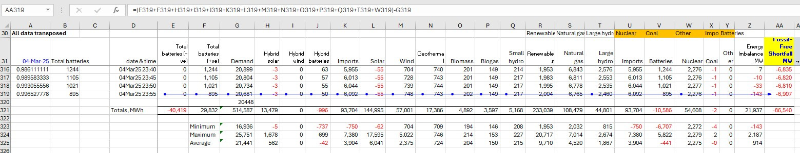
The “Fossil-Free Shortfall MW” in Column AA is the arithmetic sum of all the non-fossil power supply values minus the Demand in that time interval. Ensuring that duplicates i.e. “Renewables”, “Imports” and “Batteries” are not double-counted. The blue line’s dots show Excel’s ‘Trace Precedents’ for cell AA319, confirmed by the formula shown in the formula bar at the top of the image.
4) Battery Simulation:
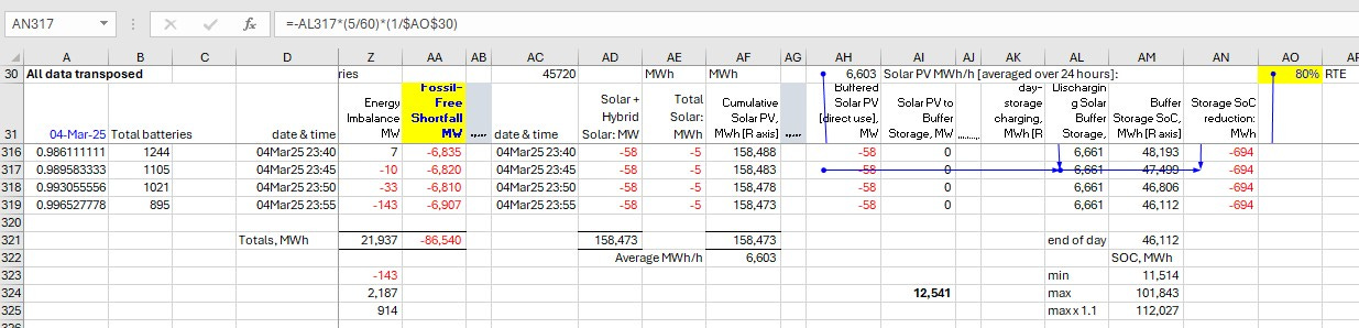
Columns AC through AO contain the battery simulation calculations to determine how large a BESS would have to be to smooth out California’s extreme daytime surge of Solar power. Column AD adds Solar and ‘hybrid Solar’ (in MW); Column AE multiplies that by 5/60 to derive the energy provided by the sun that 5-minute interval in MWh. Column AF sums all the MWh values to derive the day’s total. Cell AF322 simply divides that total by 24 to derive the average MWh/h.
Columns AH through AN contain the step-wise logical operations to determine whether Solar power is sufficiently large to charge the simulated BESS or whether the simulated BESS needs to be discharging to maintain power to the grid equal to the daily average. Column AN contains the adjustments to each interval’s BESS state of charge (SoC) to allow for energy loss per the round trip efficiency (RTE) of the BESS. Column AM then keeps track of the SoC through discharging / charging / discharging phases. Cell AM323 shows the minimum SoC that day; cell AM324 the maximum; cell AM325 = 1.1 times the maximum ~ minimum BESS capacity required; and cell AM 321 the day-end’s SoC.
Professor Jacobson inspires quite the following on Substack. Nice work Chris--thank you!
Well done, Chris - great analysis, simply stated, easy to follow, and, hopefully, makes common sense.
To that last point: having worked in the industry for over four decades as an engineer & MBA, doing everything from solving nuclear construction issues, taking R&D projects through commercialization, leading technical due diligence teams for project finance, and independently advising utility Boards on the exection status of multi-billion-dollar projects, I've lost the ability to see what makes "common sense".
You appear to have not lost that ability. In other words, this makes so much sense, I look forward to to the inane reasons and Twisted Physics* (not only weird science**, but a great band from the early '80s) people such as Prof. Jacobson will use with pretzel logic*** in trying to keep their zits intact.
* "Twisted Physics" was not a band in the early '80s as far as I know - I just made that up
** "Weird Science" is a real film from 1985 starring a young Anthony Michael Hall
*** "Pretzel Logic," is also real, a great (IMHO) Steely Dan album & song from 1974