

California Reality
Looking at real data from *the last three years* we can see what would be required to ‘decarbonise’ power generation in the Golden State

Note: in this post I explain my thinking and methodology in some detail on the basis that anyone who is reasonably adept with Excel can repeat it. My analysis uses a publicly-available data-set from the US Energy Information Agency (EIA) which anyone can download.
Please give technical feedback on any aspect of this analysis. Do you see errors in my approach? Do you replicate my results?
Also, reminder: if you view this post in Substack and want to see the detail in any of the complex charts, simply click on the image to open a zoomed view.
Additionally, Substack is warning that this post is too long for email. Yes, these complex issues require longer posts. In case of truncation please click the image in the email to see all.
Introduction
What should policy-makers do when faced with the trilemma (the triple challenges of energy security, climate change and rising geopolitical risks) of ‘decarbonisation’ of their energy grids? Many appear to begin with ‘ambitious goals’, put together a PR campaign based on those goals, set wheels in motion and hope to retire long before any impracticability becomes apparent. (Unfortunately, some policy-makers appear to believe academics who look at data from fractions of single days during a very benign time of year and assume the job is near-enough done.)
Me? I believe in data, the more the better. This is why for my recent analysis of ‘decarbonisation’ of the UK’s power generation I used four years’ continuous data from 01 January 2020 through 31 December 2023.
For this analysis of how California’s power grid might be ‘decarbonised’, I turned to the EIA’s excellent data source. Specifically I downloaded file “Region_CAL.xlsx”1 at 11:35 BST on 19 April 2024 and have been developing my analysis and writing this post since.
This particular iteration of the EIA file contains (on the ¦Published Daily Data¦ tab) complete daily sets of data beginning 2018-July-01 and ending 2024-April-16, i.e. 2,117 days. In their daily updates the EIA simply adds further rows of data in this tab, from which the pre-set lookups in the ¦Daily Charts¦ tab plot the most recent charts.
The user can define a different end-date, which is how I easily repeated my analysis for three successive years. The ¦Daily Charts¦ tab has a collection of pre-configured charts - the top five of which are shown in Figure 1 - to display the selected data. (Altogether this is a well-designed tool: thank you, EIA.)
Figure 1: EIA Charts 2023-04-18 to 2024-04-18
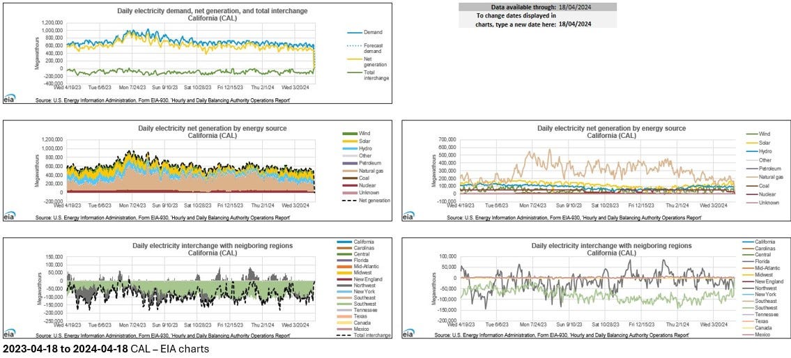
By simply summing the totals in the relevant columns on the ¦Daily Charts¦ tab and using Excel’s =MAX and =MIN functions in those columns, for this year ending April 16 2024 we can find:
- Total Demand MWh was a multiple of the total of [total Solar + Wind MWh] …
but my analysis has a bit more complexity, as I explain below;
- Total interchange with neighbouring grids was -32,377,021 MWh i.e. imported
(max daily: 12,127 MWh +ve = export; min daily: -181,219 MWh -ve = import).
- Total Nuclear was 17,632,997 MWh;
(max daily: 54,671 MWh; min daily: 2,005 MWh which appears to be a data glitch)
- Total Hydro was 32,600,306 MWh;
(max daily: 140,794 MWh; min daily: 26,763 MWh)
For my analysis I treat Nuclear and [existing] Hydro as being carbon-free and therefore to be retained in the Future CA grid. Thus I leave each data-set’s Nuclear MWh and Hydro MWh as recorded by the IEA.
In my California Dreaming post I identified that around 60% of imports are fossil-derived. In this analysis I simplify by assuming neighbouring grids will be trying to ‘decarbonise’ their own grids and thus will not want to share the power they generate. Hence I assume that in future the Interchange should average zero: in other words, future California would become electricity-independent.
To sum up: for every set of EIA daily data I calculated:
[CA In-State Net Demand] = [Demand] - [Interchange] - [Nuclear + Hydro] MWh.
Taking as an example the data for Apr 20, 2023:
D = 649,991 MWh, TI = -29,017 MWh, N + H = 163,873 MWh;
Hence in-state CA Demand = [D - TI -(NUC+WAT)]
= 649,991 - [-29,017] - 163,873 = 515,135 MWh.
And so on.
Curtailment
Currently California curtails excess power production to maintain grid stability. On every power grid, to maintain grid frequency stability, any surplus generation has to be curtailed UNLESS there is reliable AND flexible AND additional Demand connected to the grid 60/24/365 able to instantaneously absorb that surplus. Similarly in the reverse direction: to benefit from stored energy in reducing shortfalls, the storage has to be connected when the grid instantaneously needs it.2 I discuss energy storage and my approach to it below.
Figure 2: Typical CA Curtailment:
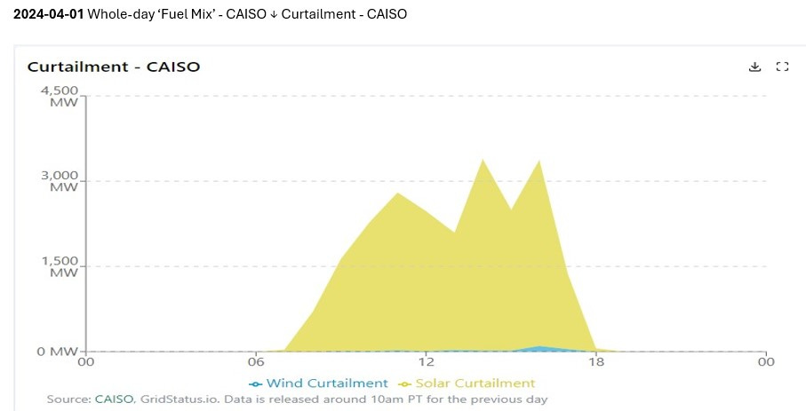
You can see from Figure 2 that CAISO curtailment is almost entirely Solar; virtually zero Wind is curtailed. Hence for simplicity I assume 100% of current curtailment is of Solar generation only.
I looked and found this monthly record of California Wind and Solar curtailments. It opens on “Wind and solar curtailment totals by month”: click on the Download button and select .csv. The file “curtailmentsMonthly.csv” contains monthly data from May/01/2014: there is no differentiation in the file between Solar or Wind being curtailed. I am confining this post’s analysis to the most-recent three years, so I focussed on the data from March 2021 as shown in Figure 3.
Figure 3: CA Curtailments Monthly
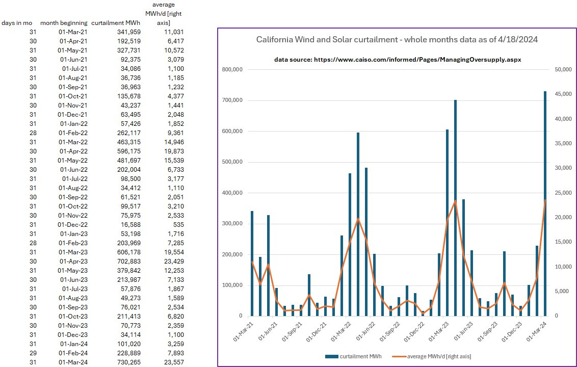
I added the days/month column, then divided Curtailed MWh (for the month) by # of days to give the MWh/d results. I copied this data table into the EIA file then used simple lookups on [month-year] for the average daily curtailment in any particular month. I then added that daily curtailment number to the EIA’s recorded MWh of Solar on that day. I prevented the Lookups from failing by assigning April 2023’s daily curtailments to April 2024. Obviously my approach is an approximation, but is close enough for my purposes.
Using the data of Apr 20, 2023 again as an example:
EIA records 145,338 MWh Solar; average curtailed Solar April 2023 is 23,429 MWh/d;
hence uncurtailed Solar that day would have been ~ 168,767 MWh.
For future California I then extrapolate from the [uncurtailed Solar] to Future Solar for each day by multiplying by the Solar multiplier.
In my Intermittency aka Diminishing Returns #2 post I explained the approach taken by the United States Department of Energy (DOE) regarding long-duration energy storage (LDES). I will make the same assumptions in this post:
- many (hundreds / thousands) of LDES facilities using a variety of technologies would have to be installed across California summing to a total Power capacity of ‘enough’ to be able to capture surplus power (subject to storage capacity and other constraints explained below);
- the round-trip efficiency (RTE) of that fleet of LDES facilities will be 60% on average. That means, for each 10 MWh of ‘renewable’ electricity captured by future CA LDES, we could get back 6 MWh. *If* all other physical constraints e.g. grid capacity could simultaneously be satisfied.
Current Energy Balance over a Year
If you accept my earlier premise that California should become energy-independent, then ∑ [Wind + uncurtailed Solar] = ∑ [CA In-State Net Demand] over each year; where each day’s
[CA In-State Net Demand] = [Demand] - [Interchange] - [Nuclear + Hydro] MWh.
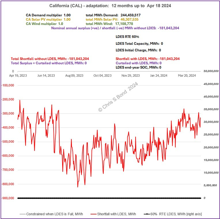
Just looking at the year ending April 16 2024 we can see how far we are from that balance:
Figure 4: 2023-04-18 to 2024-04-18 Data, In-State, Uncurtailed:
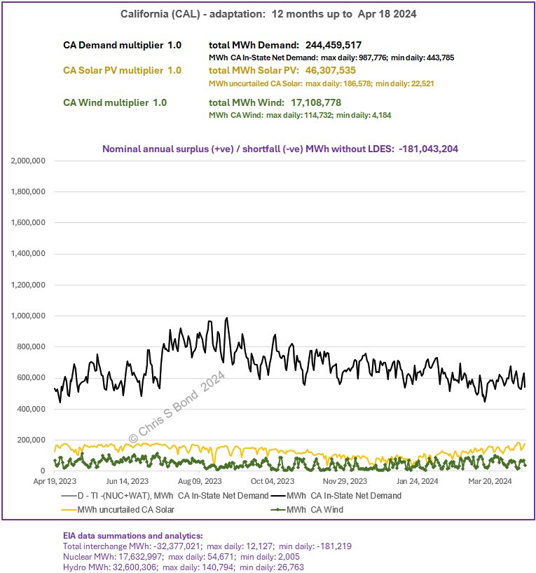
As perhaps even a Stamford Professor can see (should he ever attempt to enlighten his fan-base rather than befuddle them), California is in serious electrical energy deficit. But just in case there’s any doubt, we can plot
[Wind + uncurtailed Solar] - [CA In-State Net Demand] for every day.
If the result is positive there is a [potential] surplus;
If the result is negative there is a shortfall.
Oh look! Not one day in [potential] surplus in Figure 4A.
But how can that be? When we *know* that California is curtailing large quantities of surplus Solar, and we’ve added those quantities back in.
Obviously in the daily numbers you are averaging each day’s powers across each day’s 24 hours. Electricity doesn’t work on averages, it works on instantaneous values: if in any minute of any hour in a day there is potentially a surplus, it must be curtailed.
Figure 4A: … to 2024-04-18 In-State, Uncurtailed, Energy Balance:
If only there was a way to save surplus electricity from the good times to use in the bad.
Future California Power - Methodology
I take the EIA data and extrapolate into the future by:
- Increasing [in-state CA Demand] by the Demand factor to get [future in-state CA Demand];
- multiplying the uncurtailed Solar by the Solar multiplier to get [future uncurtailed Solar];
- multiplying Wind by the Wind multiplier to get [future Wind];
- Calculating [future Wind + future uncurtailed Solar] - [future in-state CA Demand]
As a first guess I set the Solar and Wind multipliers so as to achieve balance between [future in-state CA Demand] with [future Wind + future uncurtailed Solar] in each year. Then (down-post) I add LDES to see the effect. I assume that the Solar multiplier will be greater than the Wind multiplier since that’s already the trend in California. I don’t do financial optimisation analysis: instead I run with some example sets of parameters, as follows.
Simply by changing the year in the end-date in the EIA ¦Daily Charts¦ tab I screened three recent whole years as summarised in Table 1:
Table 1: Summary of Annual Results 2023-4, 2022-3, and 2021-2
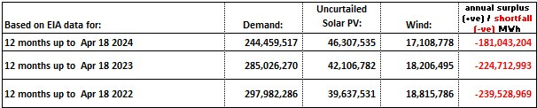
There are deficits / shortfalls of ± 200,000,000 MWh every recent year. (Note also, the Table 1 results assume that all current curtailments can be stopped, which is not currently possible.)
Running the same three years with Solar and Wind multipliers so as to approximately eliminate yearly shortfalls over the respective whole years results in Table 2:
Table 2: Extrapolation to Future Results 2023-4, 2022-3, and 2021-2
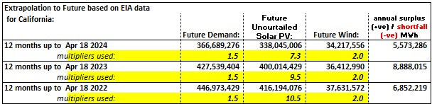
Those are the numbers averaged across the three entire years - which very definitely do NOT provide any measure of certainty that CA lights would stay on minute by minute. Also:
Is the Demand multiplier value of 1.5 realistic as California electrifies *everything*?
Would the Wind multiplier be a constant 2.0?
Who knows? But I think the size of the multipliers (7.3 times, 9½ times, and 10½ times current uncurtailed Solar *capacity*) indicates just how far CA is on average to breaking even electricity-wise.
This approach also assumes future Solar and Wind will have approximately the same load factor i.e. effectiveness as current Solar.
Looking in more detail at the latest of those years we get Figure 4:
Figure 5: Future Extrapolated from 2023-04-18 to 2024-04-18 Data,
In-State, Uncurtailed
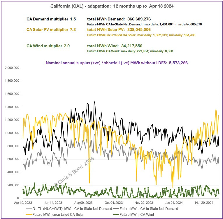
It is clear from Figure 5 that in parts of the year, future Solar alone is greater than in-State Demand, while in other parts of the year Solar + Wind falls far short of meeting Demand. We can plot the [potential] Surplus versus Shortfall chart as in Figure 5A.
Grids have to be balanced, Supply = Demand 60/24/365, so it looks like large quantities of energy storage will also be needed as well as massive additions to the Solar and Wind fleets.
Figure 5A: … to 2024-04-18 In-State, Uncurtailed, Energy Balance:
If only there was a way to save surplus electricity from the good times to use in the bad.
LDES Methodology
To emphasise: long duration energy storage (LDES) technologies do not currently exist except in infant states and/or are currently too expensive for widespread adoption at sufficient magnitude.
Even hydrogen? Yes, even hydrogen.
Even though currently LDES doesn’t exist, we can postulate that future LDES would have to operate within reality constraints as follows:
Logic Tree for Future LDES:
1 IF there is surplus [future Wind + future Solar]
2 AND there is unused energy storage capacity in future LDES
3 THEN that future LDES can receive and store ‘green’ energy (thereby reducing the
amount of energy that has to be curtailed)
4 UNTIL (at maximum) the future LDES becomes ‘full’
SO
4 WHEN there is a shortfall of [future Wind + future Solar]
5 AND there is ‘charged-up’ future LDES
6 THEN we could get back ~ 60% [1] of the energy stored in the LDES (thereby
reducing the shortfall of energy)
7 UNTIL (at minimum) the LDES becomes ‘empty’ [2]
[1] based on average round-trip efficiency per DOE
[2] The operating range of LDES needs to remain within constraints on e.g. depth of discharge (DOD) which will probably depend on its technology. I’ll work with net storage capacity and assume we remain within such constraints, whatever the technology mix.
I assume no limits on charge / discharge cycles or other aspects of LDES operation: if there is capacity to be charged, or stored energy to be discharged, then my analysis uses it.
The net effect of LDES after applying the above Logic Tree would be to reduce the size of the energy shortfalls in the future CA, and reduce curtailed quantities and hence costs. I’m making the gross simplification that all energy stored in the LDES system is equivalent to electrical power, on the basis that stored heat and coolth would unload the power system by those amounts. I understand this simplification is thermodynamically incorrect: don’t ‘@’ me.
In the process of debugging my Excel logic and fine-tuning the appearance of the graphics I was producing, I ran the three years with various levels of LDES capacity. In those trial runs I found the LDES capacity = 20,000,000 MWh gave good illustrative results, see Figures 6, 6’, 6A and 6B and Summary Table 3:
Figure 6: … to 2022-04-18 Future CA with 20,000,000 MWh of LDES:
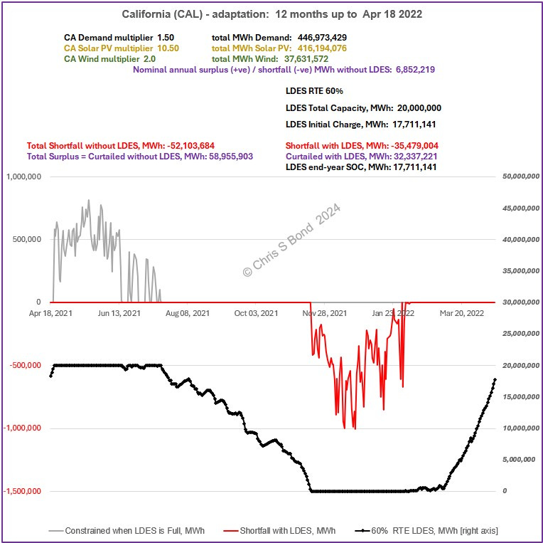
Figure 6’: … to 2022-04-18 Future CA with 20,000,000 MWh of 80% RTE LDES:
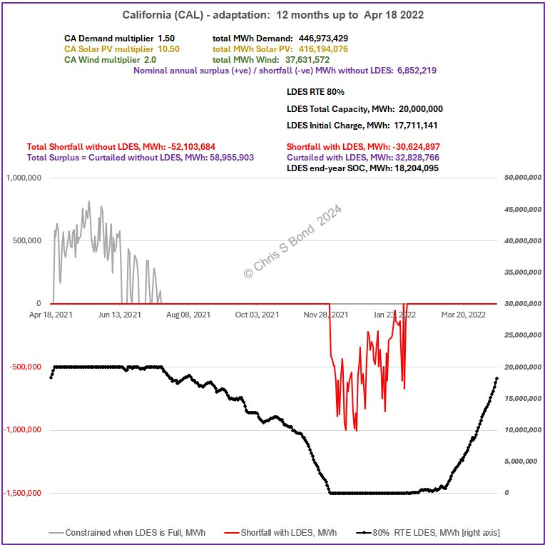
Figure 6A: … to 2023-04-18 Future CA with 20,000,000 MWh of LDES:
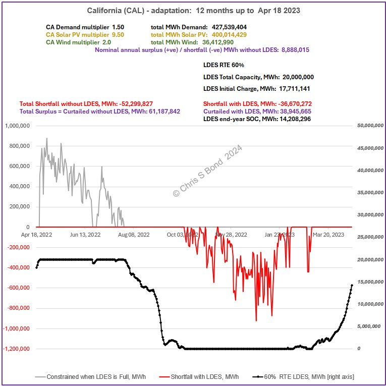
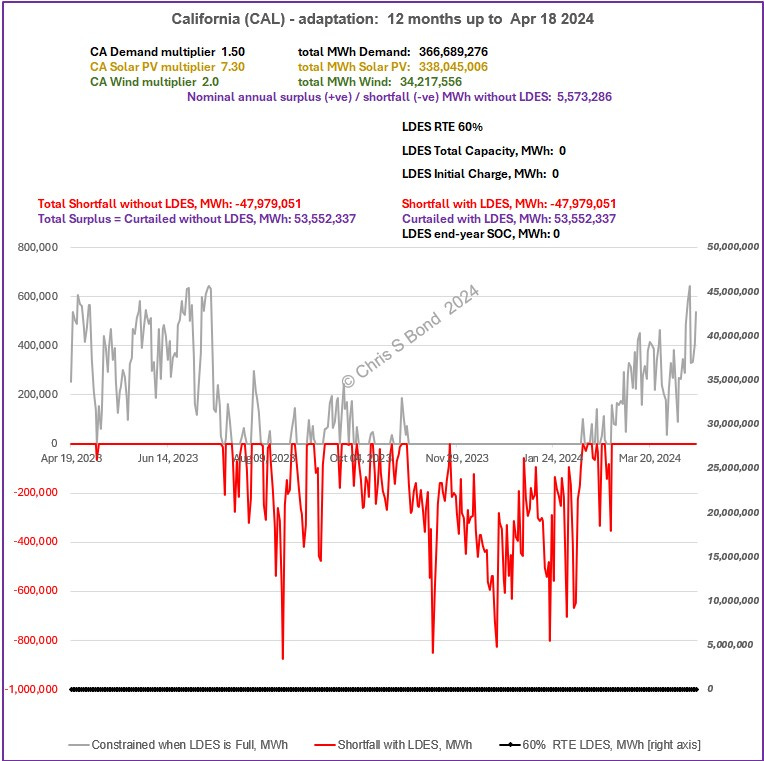
Figure 6B: … to 2024-04-18 Future CA with 20,000,000 MWh of LDES:
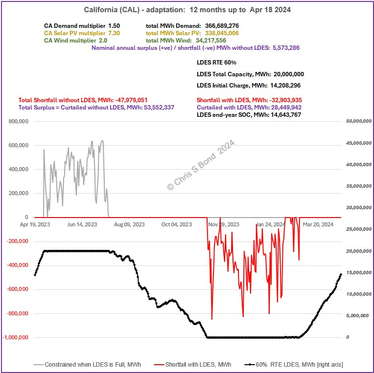
I arranged these in date order to illustrate the transfer of stored energy from the end of one year to the beginning of the next. The pattern is clear from year to year. In the benign spring conditions beginning around February each year the surplus of [future Solar + future Wind] would charge up the LDES until the LDES becomes ‘full’. Then in the less-benign summer and fall conditions the LDES discharges until it goes completely ‘flat’. The LDES stays ‘flat’ through an extended winter interval when consistent shortfalls of [future Solar + future Wind] both fail to meet future Demand and consequently fail to ‘re-charge’ the LDES. The results are summarised in Table 3.
Table 3: Summary of CA Results 2023-4, 2022-3, and 2021-2 with LDES:
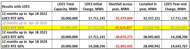
The results for each of the three years are broadly similar for the same overall LDES round trip efficiency (RTE) of 60%. The highlighted row illustrates the effect of improving storage RTE to 80%. The Curtailed quantity stays ~ the same because all surplus over the LDES capacity must be curtailed for grid stability. However, the higher LDES efficiency translates into lower losses, in other words more of the stored energy is returned to counteract the shortfalls, and so the Shortfall across a year would be significantly lower with higher efficiency LDES.3
Just How Big is 20,000,000 MWh LDES?
In a word, immense.

~ 6,000 times California’s biggest lithium-ion battery to date - which is anyway not long-duration; or
667 million 60 kWh electric vehicles constantly connected to the grid with vehicle-to-grid technology and with half their usable capacity donated to ‘the greater good’; or
Over 2,000 times Dinorwyg Pumped Hydro Storage scheme in Wales, UK (although pumped storage cannot be distributed and so would require far greater grid reinforcement to and from areas with appropriate geography); or
~80,000 times the size of a recent proposed liquid air energy storage (LAES) demonstration project... IF they can get funding. As the licensor correctly states, LAES technology has the major advantage that it can be located almost anywhere, and the energy can be stored as liquid air for extended periods.4
All of which is why chemical energy storage (e.g. as hydrogen) is seen as part of the answer to the problem of the immensity of LDES. However, round-trip efficiency using hydrogen is even lower at ~ 30-40%, and hydrogen itself is a potent greenhouse gas.
The Effect of Varying LDES Capacity
Looking at just the most recent year 2023-04-18 to 2024-04-18 I investigated the benefits of different capacities of LDES systems.
Table 4: Summary of CA Results 2023-4 with Varying LDES:
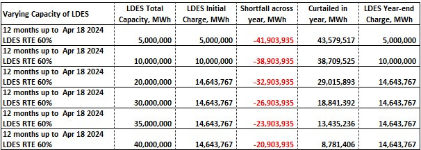
From the charts we see that California has a long ‘charging-up’ season each spring followed by a long ‘discharging’ season each summer and fall, with a ‘flat’ season through winter. Given the Demand, Wind and Solar multiples I have used, greater LDES total capacities result in virtually 1:1 reductions in Curtailed MWh. Note also that with this set of parameters and for these years the LDES goes ‘flat’ every winter.
Figure 7: … to 2024-04-18 Future CA with 30,000,000 MWh of LDES:
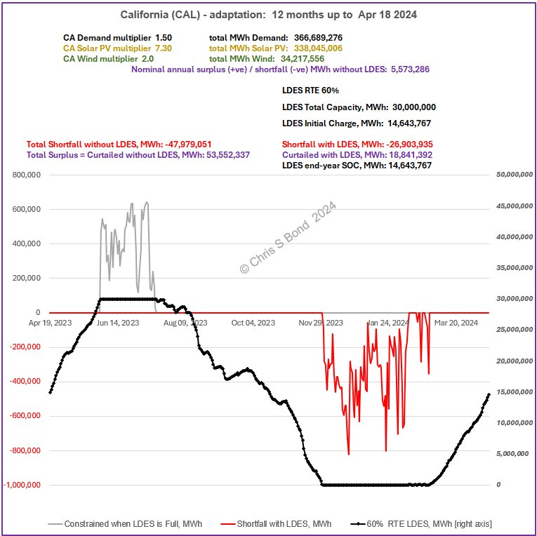
Figure 8: … to 2024-04-18 Future CA with 40,000,000 MWh of LDES:
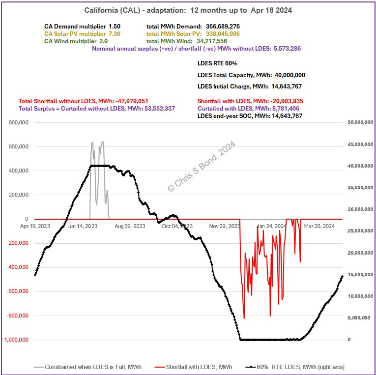
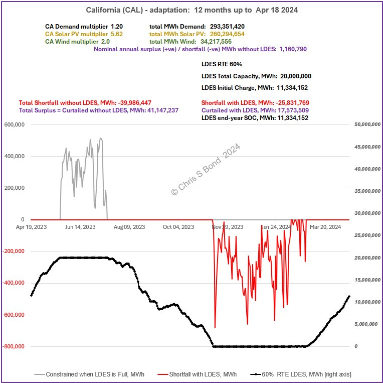
A Lower-Demand Future California
What if future Demand is lower than I have assumed? Then we would need smaller multipliers to achieve overall energy balance.
For example, for the year ending 2024-04-18, if the Demand multiplier is 1.2 times then we can achieve overall energy balance by applying a multiplier of 5.62 to the uncurtailed Solar, while keeping the Wind multiplier at 2.0 as before. Then, with a total LDES capacity of 20,000,000 MWh with RTE 60% we get the chart shown in Figure 9:
Figure 9: … 2024-04-18, Lower Demand CA, 20,000,000 MWh of LDES:
Conclusions
Only by looking at large amounts of continuous real data (2-3 years) is it possible to develop an informed opinion on how close any territory (even California) is to being able to run solely on weather-dependent power generation.
For California the multiples of Solar and Wind *capacity* required to even approach energy sufficiency are very large (~7 to 11 times) and large (2 times) respectively if we assume Demand increases by a factor 1.5.
California is already curtailing large amounts of mainly Solar energy. To avoid having to curtail more and more, California needs to install reliable AND flexible AND additional Demand, probably in the form of long-duration energy storage (LDES). But the capacities of LDES required to make a significant difference are truly immense: for example, up to 40,000,000 MWh was included in this analysis and still did not fully prevent curtailments.
Copyright © 2024 Chris S Bond
Disclaimer: Opinions expressed are solely my own.
This material is not peer-reviewed.
I am against #GroupThink.
Your feedback via polite factual comments / reasoned arguments welcome.
I also downloaded file “CISO.xlsx” and compared the daily charts from both, side-by-side.
Here the daily charts from file “CISO.xlsx” [~72MB]:
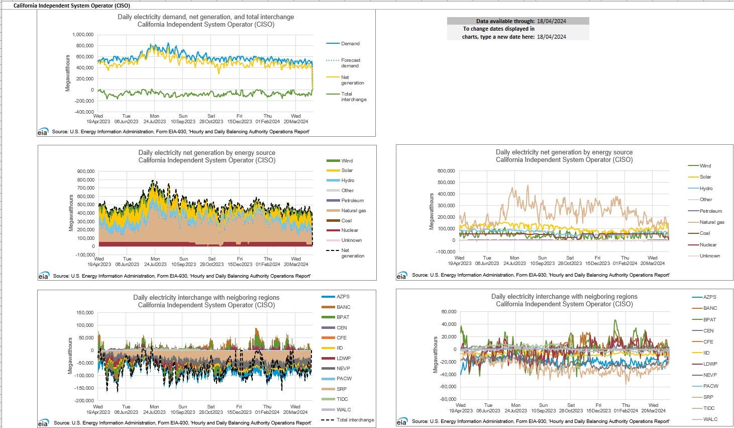
… and here from “Region_CAL.xlsx” [~27MB]:
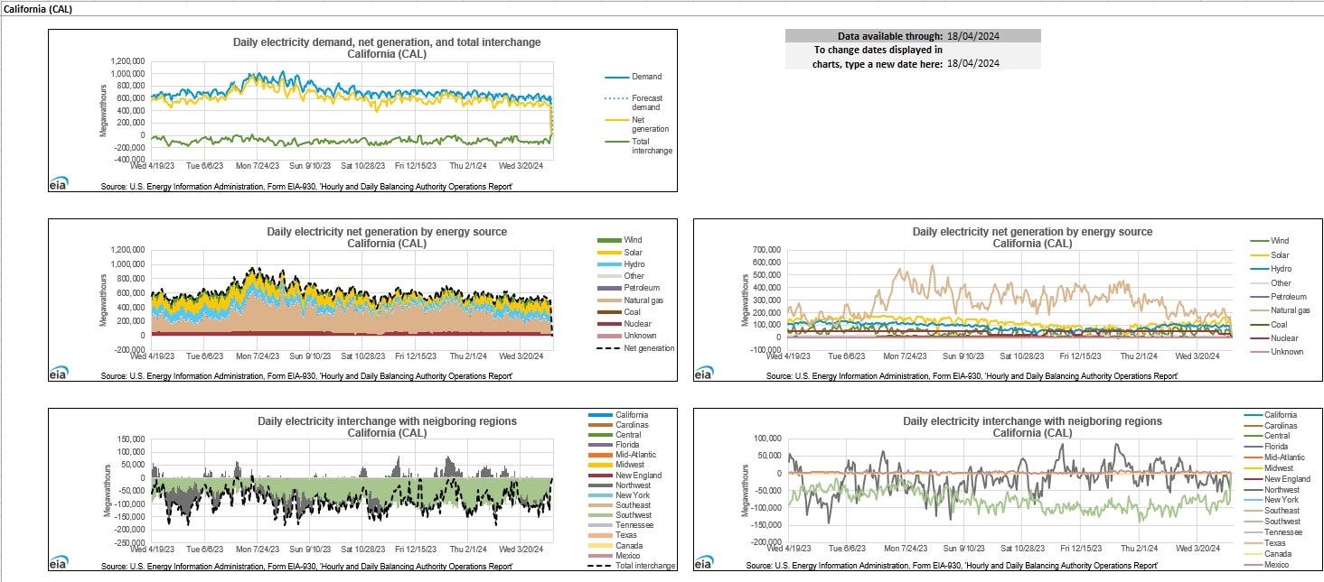
I cannot see a material difference between them, and the CISO file is nearly 3 times larger. So I chose to use the smaller “Region_CAL.xlsx” file as the basis for my analysis.
Fans of vehicle-to-grid (V2G) technology seem to think this does not require vehicles to be plugged in continuously, but I don’t see how that’s possible. I’ve yet to receive a convincing explanation as to how this particular conundrum can be solved.
I choose to use the ¦Daily Charts¦ for convenience and to facilitate replication if others would like to give it a go. The disadvantage of this is that I am working on only 364 sets of data. Any rounding or truncation errors in my logic calculations in this relatively small data-set therefore become slightly more significant as compared with my UK analysis (which used ~105,000 lines of data each year). However, I am confident it gives a broadly accurate ‘big picture’ view for California.
A downside of cryogenic processes is that they have to be kept intensely cold, unlikely if they are reliant solely on surplus ‘renewable’ power. So it will be interesting to watch as experience is developed revealing the overall efficiency and economics of LAES facilities.