
Diminishing Returns #2 - DIY Kit
Diminishing Returns #2 - DIY Kit
The Geek's Guide to replicating my analyses - I hope

Introduction
My Intermittency aka Diminishing Returns #2 post has received quite a bit attention, thank you All! But I’m sure there’s some scepticism as to my methodology. Hence I expect my conclusions are dismissed by some who prefer to keep their comforting beliefs about the practicability of the energy ‘transition’ unsullied by uncomfortable information. So I thought I would put together this ‘Geek’s Guide’ for assembling your own version of the analysis. I am keen to receive constructive feedback and I hope to see someone replicate my results.
I use Excel to convert the raw data, crunch all the numbers and plot the charts. As I frequently mention, I use GridWatch data. (If you do too, please contribute to their running costs via the [Donate] button, I think they perform an invaluable service.)
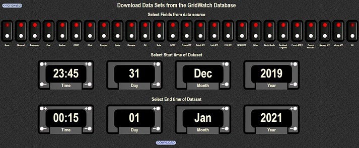
The [Download] button opens access to the full database beginning 13 May 2011.
WARNING: Do NOT download more than 1 year’s data at a time!
Each year’s raw data is about 20MB / 105,000 lines. For reference, my finished Excel files with the calculations, logic and plots ended up around 60MB for each whole year.
Figure 1: GridWatch Download settings for all of 2020 (as an example)
I apologise in advance to any experienced Excel users for ‘teaching my grandparent to suck eggs’, but in this ‘Geeks Guide’ I’m going through each step in full detail. That way I hope any errors I’ve made will be easier to spot / more people can hopefully have a go themselves and feed back to me if they can replicate my results.
Also please note: where I’ve documented my working in other posts, rather than repeat that documentation every time I’ve mostly linked to that specific part of the previous post (a very neat feature of the Substack environment).
The downloaded file from Gridwatch is in ‘comma-separated variable’ (.csv) format and is always named “gridwatch.csv”. I tend to rename the file with the date range, e.g.
“gridwatch raw Jan2020.csv” to facilitate later access if needed: for example, to re-load the raw data into the ‘data landing area’ of a better version of the template Excel file.
Open a .csv file in Excel and the app will convert the data to unformatted rows and columns. The first time you do this use File, Save As to save it as an Excel file (.xlsx) to preserve all formatting, plotting, etc. I suggest you use this first Excel file as the template for other data date ranges by keeping the ‘data landing area’ unchanged. That is, keep all number manipulations, logic calculations, etc. etc. to a range of cells offset from the ‘data landing area’. See Figure 2.
Figure 2: ‘data landing area’ vs calculations areas

Once you’ve programmed and debugged the template1 you can File, Save As using an appropriate (and hopefully informative) filename. Then you can load the template with another date-range’s raw data-set by copying from the full data range of the next .csv file then pasting into the template’s ‘data landing area’: in my example this begins at cell A17.
Tip 1: to select a large range of data (e.g. from the downloaded .csv file), select the top left data cell i.e. 1 row down from the heading row; hold the [Shift] key down and keep holding it down; hit [End] [down] then [End] [right]; release [Shift]. Then [Ctrl]-[C] to copy. Then move to the window with your template file, select the top left cell in its ‘data landing area’ (cell A17 in my example), then [Ctrl]-[V] to paste.
Tip 2: leave an empty column between the ‘data landing area’ and the start of the number-crunching area. [End] [right] will then stop at the gap.
Tip 3: put plots onto a separate tab in the template: that makes them much easier to find, edit, etc.
Tip 4: do all fine-tuning, debugging, plotting, etc. in your template. But see footnote 1.
For the example programming below I have chosen a middle-of-the-day data-set to ensure that most parameters including Solar PV have non-zero values.
The Calculations
a) Optional - active date and time
I prefer to plot the data with actual dates & times along the X-axis. Gridwatch stores that information in text format under the “Timestamp” column B in a ‘raw’ data-file.
e.g. cell B160 of my 2023 file has text string “ 2023-01-01 11:55:42” which begins with a space and has the date in YYYY-MM-DD format.
To fully convert this text string to an Excel data and time takes 4 operations:
1. date text =LEFT($B160,11) result “ 2023-01-01” in cell AB160;
2. date =RIGHT(AB160,10) result “2023-01-01” in cell AC160;
3. time =RIGHT($B160,8) result 11:55:42 in cell AD160;
4. date and time =AC160+AD160 result “2023-01-01 11:55” in cell AE160 2
Column AE can then be defined as the origin of the X-values of X-Y plots, with columns containing the results of [future power flows] to define sets of Y-values.
If you don’t perform this date & time conversion, plots can still be produced using Column B “timestamp”, but the X-axis will simply be numbered [e.g. 1-105,000(-ish) for a full year.]
b) Demand multiplication factor
In the electrified future, electricity Demand is forecast to be higher. According to this February 10, 2022 McKinsey article, it will be 56% higher. For simplicity I assume that ties in with the end-point of Labour’s Climate ‘Mission’ i.e. by December 2030.
c) Wind and Solar PV Adjustment factors
I explained my rationale for the Wind and Solar PV Adjustment factors in this part of my ‘Diminishing Returns’ post, and summarised the results for recent years in this section of my ‘Intermittency aka Diminishing Returns #2’ post.
D) Demand multiplication factor
This is the part of my analysis which I think is most open to interpretation. There is uncertainty because we have actual installed capacities of Onshore Wind, Offshore Wind and Solar PV for recent years as I included here. But Labour’s ‘Mission’ has different proportions of the two types of Wind. Plus, I’ve tried to give credit for future expected technology improvements as I summarised here. So I’m extrapolating from known recorded data using slightly uncertain future factors. But, as they say, forecasting the future is difficult.
After that last linked section I included this text: “I suspect some ‘renewables’ proponents will claim higher increases, but I think we need some operational / maintenance / breakdown history for some of these novel / massive structures and machines before we can confidently assume more-optimistic numbers.”
Now that I’m gathering this all together I also realise that none of those improvements in load factor will be available overnight: instead they are likely to ramp up over time, so I have more confidence in using less-optimistic numbers.
Hence I get Wind multipliers for predicting end-of-2030 Wind power generation:
4.23 with 2020 Gridwatch data
4.58 with 2021 Gridwatch data
3.73 with 2022 & with 2023 Gridwatch data
And Solar PV multipliers for predicting end-of-2030 Solar power generation:
3.90 with 2020 Gridwatch data
3.96 with 2021 Gridwatch data
3.58 with 2022 and with 2023 Gridwatch data
E) Methodology
The heading is a link but I’ll repeat the text here:
For GridWatch data from each of those years [2020, 2021, 2022 & 2023] I extrapolate to end-2030 by:
- Adjusting recorded Wind power flows by the Wind adjustment factor, then
multiplying the adjusted Wind by the Wind multiplier to get [future Wind];
- Adjusting recorded Solar PV power flows by the Solar adjustment factor, then
multiplying the adjusted Solar by the Solar multiplier to get [future Solar];
- Increasing the recorded Demand by the Demand factor to get [future Demand];
- Calculating [future Wind + future Solar] - [future Demand]
Simplistically, if [future Wind + future Solar] - [future Demand] is greater than zero, the future UK is more or less energy-independent and the UK’s lights will stay on.
However, if [future Wind + future Solar] - [future Demand] is less than zero, the future UK is NOT energy-independent. Depending on what third parties decide to do, the UK’s lights may or may not stay on.
In Excel (examples below showing numeric values for use with 2022 or 2023 data; running other years of data require the appropriate numeric values):
Set cell AF6 =1.56 (future Demand factor);
Set cell AG3 =1.268 (Wind adjustment factor);
Set cell AG6 =3.73 (Wind multiplier);
Set cell AH3 =1.165 (Solar adjustment factor);
Set cell AH6 =3.58 (Solar multiplier)
Then again e.g. on row 160 with the data-set for 2023-01-01 11:55:42:
Demand (cell C160) = 26880 (downloaded from GridWatch)
Future Demand D' (cell AF160) =$C160*$AF$6 =26880*1.56 =41,933 (MW)
Wind (cell H160) = 9782 (downloaded from GridWatch)
Future Wind W' (cell AG160) =$H160*$AG$3*$AG$6 =9782*1.268*3.73 =46,291 (MW)
Solar (cell M160) = 1316.61 (downloaded from GridWatch)
Future Solar S' (cell AH160) =$H160*$AH$3*$AH$6 =1316.61*1.165*3.58 =5,497 (MW)
Plotting Columns AF , AG and AH against ‘live date & time’ Column AE as an X-Y Scatter plot / alternatively text date & time Column B / produces the basic plots of Future Demand D’ MW [format black], Future Wind W' MW [format blue] and Future Solar S' MW [format yellow].
Column AJ is headed “[potential] Surplus MW when W' + S' > D' ” in cell AJ13
For row 160: =IF((AG160+AH160)>AF160,(AG160+AH160-AF160),0)
Substituting the results from above:
IF((46,291 +5,497)>41,933,[true hence] 46,291 +5,497 -41,933) i.e. cell AJ160 = 9,855
Column AK is headed “Shortfall MW when D' > W' + S' ” in cell AK13
For row 160: =IF((AG160+AH160)>=AF160,0,(AG160+AH160-AF160))
Substituting the results from above:
IF((46,291 +5,497)>=41,933,[true = 0],) i.e. cell AK160 = 0
Plotting Columns AJ and AK against ‘live date & time’ Column AE as an X-Y Scatter plot / alternatively text date & time Column B / produces the basic plots of future [potential] Surplus MW [format grey] and future Shortfall MW [format red].
To emphasise why that is only “[potential] Surplus”. For grid frequency stability to be maintained, any surplus generation has to be constrained / curtailed UNLESS there is reliable AND flexible AND additional Demand connected to the grid 60/24/365 able to instantaneously absorb it. Similarly in the reverse direction if there’s to be benefit from stored energy in reducing shortfalls. Fans of vehicle-to-grid (V2G) technology seem to think this does not require vehicles to be plugged in continuously, but I don’t see how that’s possible. I’ve yet to receive a convincing explanation as to how this particular conundrum can be solved.
F) Programming The Logic Tree for Future LDES
I covered the approach I’m taking to long-duration energy storage (LDES) here.
In the Excel example I set the following parameters:
Long Duration Energy Storage (LDES) systems design capacity, MWh: cell X5
LDES round-trip efficiency, %: cell X6
/optional LDES start-year stored energy, MWh: cell X7
IF the previous year’s analysis results in energy remaining in LDES at the end of 31 Dec.
But I found it made little difference with the 2020-2023 years. /
A couple of the logical constraints on LDES - the energy stored cannot go below zero and it cannot go above the maximum available LDES capacity - could potentially lead to circular [fatal error] calculations in Excel. I got around this by performing the logical tests for a particular time interval on the results for the previous time interval. The time intervals in Gridwatch are 5 minutes = 1/12th of an hour so I don’t think this introduces significant inaccuracies for the majority of possible analyses.
However, I did notice that as you approach the upper limit of LDES capacity while still retaining minimal shortfall - the 2030 GB, 2023 Actual Weather, 7,300,000 MWh LDES case, Figure 3 - the ratio of [reduction in shortfall] to [reduction in constrained power] was 32.1 / 60.6 i.e. ~53%, whereas for all the lesser LDES capacities included in that post that ratio was 60% = round-trip efficiency of the LDES.
To continue with the logic tree programming and for the moment still staying with row 160. But realising that the results of the logic tree in terms of the ‘state of charge’ of the LDES only become apparent when you run tens of thousands of lines of data through the code.
Column AM heading in cell AM13 is “Surplus MWh when W' + S' > D'”
Column AN heading in cell AN13 is “Shortfall MWh (no LDES) when D' > W' + S'”
These simply convert the MW power results from columns AJ and AK by multiplying by 5/60 h per interval;
i.e. AM160 is =AJ160*5/60 =9,855*5/60 = 821 [display formatted to zero decimals]
i.e. AN160 is =AK160*5/60 =0*5/60 = 0 [display formatted to zero decimals]
Last key column headings:
Column AQ cell AQ13 is “60% RTE LDES energy opposing shortfall MWh”
Column AR cell AR13 is “Net Stored MWh in 60% RTE LDES”
Column AS cell AS13 is “Net shortfall MWh (with LDES) when D' > W' + S'”
Column AT cell AT13 is “Net Stored MWh in 60% RTE LDES (right axis)”
Column AU cell AU13 is
“Net surplus = Constrained MWh when W' + S' > D' after charging LDES”
Remembering we need to avoid circular reference fatal errors as noted above:
cell AQ160 =IF(AR159>0,IF((AM160+AN160)<0,(1/$X$6)*AN160,0),0)
i.e. only if there is stored energy in the previous interval’s LDES (AR159) and only if there is a shortfall this interval [AM160+AN160)<0] will you effectively discharge the LDES by (1/60% = 1.67) times the shortfall AN160
cell AR160 =MIN($X$5,MAX(0,IF(AM160>0,AM160+AR159+AQ159,AR159+AQ159)))
value is constrained between maximum design capacity of LDES $X$5 and zero.
If this interval’s surplus AM160 is greater than zero it is added to the previous interval’s LDES stored energy AR159 plus any [negative] energy used to oppose the previous interval’s shortfall AQ159;
otherwise it’s just the previous interval’s LDES stored energy AR159 plus any [negative] energy used to oppose the previous interval’s shortfall AQ159
cell AS160 =IF(AT160>0,0,AN160) keeps the count of MWh shortfall after LDES action
cell AT160 =IF(AR160>$X$5,$X$5,AR160) constraint of maximum design capacity of LDES $X$5 and Column AT is used for plotting
cell AU160 =IF(AT159>=$X$5,AM160,0) keeps a count of MWh that has to be constrained / curtailed
G) Final Touches
If you plan ahead with the template, for example first load it with whole-year 2020 (which is a leap year) you will find that the raw data-file has around 105,410 rows. Therefore any manipulations on whole columns of data, or automation of chart annotations using text concatenation, should avoid being in rows 14-105,423. I also find it useful to have an occupied ‘last row’ at the bottom so I can used [End][down] two or three times and get to it painlessly. Hence
Cell AF105426 “ max Future Demand ” label
Cell AF105427 =MAX(AF15:AF105425) => the maximum value of Future Demand D’
For 2023 data this = 73,269 MW
Manually use Excel Search [Ctrl]-[S], Within Sheet, By Columns, Look in Values in Column AF, remembering (if you’ve formatted it with comma separators as I have) that the search string is “73,269”: you find this value in cell AF98057 which has the live date and time 07/12/23 17:41 in AE98057.
Then manually set AK105431 =AE98057
Convert this into text in your desired format e.g. in
cell AM105431 ="{"&TEXT(AK105431,"dd mmm 'yy hh:mm")&"}" ={07 Dec '23 17:41}
Then cell AF105431 =AF105426&TEXT(AF105427,"#,##0")&" MW "&AM105431 =
“ max Future Demand 73,269 MW {07 Dec '23 17:41}”
Then if you make your plot transparent [zero fill] you can display this through the plot by a calculation of the form ='gridwatch raw'!$AF$105431
when the number-crunching is on the ¦gridwatch raw¦ tab and plots are on e.g. the ¦charts¦ tab:

And so on.
AM1 Shortfall MWh (no LDES) when D' > W' + S' =SUM(AN14:AN105424)
AM2 Net shortfall MWh (with LDES) when D' > W' + S' =SUM(AS14:AS105424)
AM3 Max possible reduction in shortfall from LDES this year =AM2-AM1
AU1 Net constrained =SUM(AU14:AU105424)
AU2 Constrained without LDES =SUM(AM14:AM105424)
AU3 Net reduction in constrained power with LDES =AU2-AU1
Now over to you.
Your mission, should you choose to accept it, etc. etc.
Please *do* let me know what results you get if you have a bash.
Copyright © 2024 Chris S Bond
Disclaimer: Opinions expressed are solely my own.
This material is not peer-reviewed.
I am against #GroupThink.
Your feedback via polite factual comments / reasoned arguments welcome.
You will probably find this is an iterative process. Each downloaded .csv file has a different number of rows, produces different maximum values of parameters you’re plotting, and so on. I strongly recommend you NOT to do different programming in different versions of Excel files - that way will end up with you rapidly getting tied in knots. Instead, be prepared to load different data-sets into the one template, see what results you get, reset e.g. plot scales accordingly, then only keep one master Excel file and re-load it with other sets of raw .csv data. For example, I am particular to keep plot scales the same across years so honest and clear comparisons can be made between figures: often the only way to find what are the limits needed for plots is by loading in all the sets of data one after the other to see.
I do in this post strongly suggest starting with a leap year’s data because that will set where the bottom rows will be. Subsequent data-sets will have fewer rows active: simply delete the contents of cells containing data and calculations that are not relevant. DO NOT DELETE ROWS.
Warning for anyone doing this on a US-format machine: your version of Excel may impose American date format (MMDDYYYY) on the interpretation of dates.
Hi Chris.
A most helpful guide, thanks for detailing your processes.
Gotta love your "WARNING: Do NOT download more than 1 year’s data at a time!" Yup, if all generation sources are selected, then at 5-minute intervals the resultant file is massive.
A few years ago I did a simple analysis of just one year's Wind vs Demand.
To make the data & file-size more manageable I culled 5 out of every 6 rows to represent ½-hourly settlement periods.
Then, I sorted the 'Wind' column Min>Max to trap a few examples of 'Zero'.
Those rows were temporarily colour-coded. Rows were resorted on Time/Date and the coloured Zeros manually infilled with a simple average between previous and subsequent non-zero readings.
That was sufficient for my needs of visually highlighting just how wildly variable the combined output of our fleet of geographically dispersed metered turbines is - on a per Settlement Period basis.
It showed that the claim "The wind is always blowing somewhere" was technically correct, but pragmatically near to useless.
Then along came Elexon's interactive Insights Solutions
https://bmrs.elexon.co.uk/generation-by-fuel-type
It's not as finely tuneable as data from Gridwatch, but it saves a significant number of keystrokes and can produce a reasonable chart in less than a minute.
Kind regards.